
BDM Development - your first bdm class in Matlab
bdmtoolbox provides a prodefined points of extensions in directory applications/bdmtoolbox/mex/mex_classes.The easiest way to extend bdmtoolbox is to use clasess starting with "mex". The simplies class of this type is mexFnc, which just contains name of an arbitrary matlab function to call. See Pdfs with functional transformation example.
This tutorial assumes you are familiar with basic classes of BDM: pdfs, random variables (BDM Use - Probability density functions) and estimators (BDM Use - Estimation and Bayes Rule).
Previous part of the tutorial introduced ways how to use existing classes. If no premade class is suitable for your mneeds, you can create your own class in Matlab via predefined interfaces to class epdf (mexEpdf) and BM (mexBM). These classes are treated as regular C++ classes in prepared mex files. Creation of a new estimator (offspring of class BM) can be achieved by inheriting from class mexBM.
In practice this means creation of a new file, e.g. my_bm.m, with header:
class my_bm < mexBM
Creating your own probability density
Creation of your own density is achieved by inheriting from mexEpdf:class my_pdf < mexEpdf
Calling methods from mexEpdf will result in an error that tells you which functionality is missing. It is necessary to give them a meaning.
Epdf is a class representing probability density function of a multivariate (vector) variable.
The easiest example of a density is dirac Delta function
![\[ f(x_t) = \delta( x_t - \bar{x}_t ) \]](form_269.png)
with properties:
 is the statistics of this density.
- dimension of the density is dimension of the vector
- the mean value of the density is

- the variance value of the density is
- all samples from this density are equal to
These properties are encoded in software as follows:
classdef mexDirac < mexEpdf
    % Dirac delta probability distribution
    properties                                                 % DATA structures
        point                                                  % point of the support, \bar{x}_t
    end
    methods
        function m=mean(obj)                                   % compute mean values of the density
            m = obj.point;
        end
        function obj=validate(obj)                             % check if data structures are consistent
            % point should be a column
            if (size(obj.point,2)>1)
                if (size(obj.point,1)==1) % it is row
                    obj.point = obj.point';
                end
            else
                error('Point in mexDirac is not a vector');
            end
        end
        function dim=dimension(obj)                            % inform others about your dimensions
            dim = size(obj.point,1);
        end
        function v=variance(obj)                               % compute variance
            v=zeros(size(obj.point));
        end
        function l=evallog(obj,x)                              % return logarithm of your density at point x
            if obj.point==x
                l = inf;
            else
                l=0;
            end
        end
        function s=sample(obj);                                % return random sample from your density
            s = obj.point;
        end
    end
end
An additional compulsory function is called validate which is called always before use of the class in an algorithm. The task of this function is to detect any inconsistency in the object and give the user an appropriate warning. For example, in this case, the function checks if the property point is indeed a vector and not a matrix or other structure.
Once you define the methdos above, this object can be plugged into (almost) an arbitrary algoritm, such as simulator, etc.
For seamless use with other objects, you need to define its random variables - via attribute rv, Using built-in pdfs.
For inspiration see example class mexLaplace.m and its use in simulation in tutorial/userguide/epdfds_example.m
Defining your own Bayesian Estimator (BM)
If you look into the mexBM.m file you see the basic attributes and default functions. mexBM as such will not work as a valid estimator. In order to make it work, you need to re-define at least functions dimensions and bayes, and attribute apost_pdf:This function announces sizes of random variables to other objects.
These sizes can be fixed for a specific problem, or derived from size of internal objects. E.g. for a Kalman filter, the function would be:
function dims=dimensions(p)
   %please fill
   %dims = [size_of_posterior size_of_data size_of_condition]
   dims = [size(A,1), size(C,1), size(B,2)] %
end
 is the rows of matrix A, size of
  is the rows of matrix C and the size of
  is given by columns of matrix B.
The argument apost_pdf should be a valid object of class mexEpdf, see previous section how to achieve it.
The second function to extend is
function obj=bayes(obj,dt,cond)
   % transform old estimate into new estimate
end
Here, you need to define an update (both time- and data-update) of your Bayesian filter.
Note, that statistics of the posterior are stored in attribute apost_pdf. So, the task of this function is to update fileds in apost_pdf.
Any additional attributes needed for this task shoul be added to properties of the object.
Example task: Laplace estimation
Consider a systems, where data are generated by a Laplace model
![\[ f(y_t|a,b) = \frac{1}{2b} \exp \left( -\frac{x-a}{b} \right) \]](form_273.png)
with unknown time-varying parameters  and
and  .
.
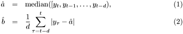
We decided to estimate parameters of the system using ML estimates of parameters on a sliding window. The estimates are then:
Implementing this system in BDM requires the following steps:
- realize that ML estimation is an extreme approximation of Bayes rule with posterior in the form of Dirac delat pdf, this pdf is ready from the previous step.
- under this choice, the posterior is a 2-dimensional dirac, which is encoded as:
 apost_pdf = mexDirac;
 apost_pdf.point = [0;0];
- the class mexDirac as introduced has only one attribute: point, which is a vector of the support. If we wish to distinguish the meaning of these values, we use attribute rv. For example,
apost_pdf.rv = RV({'a','b'}); - the class representing an estimator of this type, needs to remember internal statistics in the form window of data, which will be stored in properties of the class
- dimensionality of the estimator is then: 2-dimensional parameters, 1-dimensional observation, 0-dimensional conditioning variables. It is encoded as:
function dims=dimensions(p) %please fill %dims = [size_of_posterior size_of_data size_of_condition] dims = [2,1,0] % end - the method
bayesthen copies the obtained data into the window and updates estimates
This estimator has been implemented as class mexLaplaceBM as follows:
This is implemented as follows:
classdef mexLaplaceBM < mexBM
    % Approximate Bayesian estimator of parameters of Laplace distributed observation.
    % Maximum likelihood approximation of the Bayes rule is used, posterior is in the form of dirac.
    properties
        max_window_length = 10;                               % max window length (default = 10)
        data_window =[];                                      % sliding window of data
    end
    methods
        function obj=validate(obj)                            % prepare all internal objects for use
            obj.apost_pdf = mexDirac;
            obj.apost_pdf.point = [0;0];
            obj.log_evidence = 0;                             % evidence is not computed!
        end
        function dims=dimensions(obj)
            %please fill: dims = [size_of_posterior size_of_data size_of_condition]
            dims = [2,1,0]                                    % we have: [2d parameters, 1d observations, 0d condition]
        end
        function obj=bayes(obj,dt,cond)                       % approximate bayes rule
            if size(obj.data_window,2)>=obj.max_window_length
                obj.data_window = [dt obj.data_window(1:end-1)];
            else
                obj.data_window = [dt obj.data_window];
            end
            % transform old estimate into new estimate
            m_hat = mean(obj.data_window);
            b_hat = sum(abs(obj.data_window-m_hat))/ size(obj.data_window,2);
            obj.apost_pdf.point = [m_hat; b_hat];             % store result in psoterior pdf
        end
    end
end
Alternative representations of this estimator
Note, that the estimator above is rather coarse approximation of the Bayes rule. Indeed, in this case, the sliding window represnts a statistics on the posterior parameters, and thus it should be part of the posterior, which can thus evaluate more moments that the current Dirac density.Such a design is certainly possible, however, it would result in much more complex calculations and more complex coding. If that is the aim, a new class can be designed.
Predictors and simulation
Note, that the Laplacian likelihood model of the example is not needed for its estimation. The very basic estimator introduced above does not need to know about existence of the likelihood function.However, existence of this distribution is required by related tasks of data simulation and data prediction. Therefore, a class mexLaplace was designed, which implements all operations of pdf in the same manner as the in Creating your own probability density.
This pdf is then used in the mexLaplaceBM in function that creates predictors:
function p=epredictor(obj,cond)                       % when predictive density is needed approximate it by Laplace with point estimates
   % return predictive density (max likelihood)
   p = mexLaplace;
   p.mu = obj.apost_pdf.point(1);
   p.b  = obj.apost_pdf.point(2);
        % do not forget to validate
   p=p.validate;
        % assign descriptions
        p.rv = yrv;
        % rvc is empty be default
end
Also, the class mexLaplace can be used to generate data, see bdmtoolbox/mex/epdfds_example.m
Since it provides all required methods, it can be combined with other pdfs in chain rules, as in pdfds_example.m
Similar extensions to mexEpdf and mexBM can be made to other classes. See library/mex/mex_Epdf.h and library/mex/mex_BM.h how it is done. As always, feel free to contact the maintainer for help.
Generated on 2 Dec 2013 for mixpp by
 1.4.7
1.4.7