
BDM Use - Estimation and Bayes Rule
Bayesian theory is predominantly used in system identification, or estimation problems. This section is concerned with recursive estimation, as implemented in prepared scenarioestimator.Table of contents: Bayes rule and estimation Estimation of ARX models Model selection Composition of estimators Matlab extensions of the Bayesian estimators
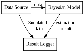
The function of the estimator is graphically illustrated:
Here,
- Data Source is an object (class DS) providing sequential data,
![$ [d_1, d_2, \ldots d_t] $](form_153.png) .
. - Bayesian Model is an object (class BM) performing Bayesian filtering,
- Result Logger is an object (class logger) dedicated to storing important data from the experiment.
Bayesian Model (bdm::BM).Bayes rule and estimation
The object bdm::BM is basic software image of the Bayes rule:
![\[ f(x_t|d_1\ldots d_t) \propto f(d_t|x_t,d_1\ldots d_{t-1}) f(x_t| d_1\ldots d_{t-1}) \]](form_154.png)
Since this operation can not be defined universally, the object is defined as abstract class with methods for:
- Bayes rule as defined above, operation bdm::BM::bayes() which expects to get the current data record
dt,
- evidence i.e. numerical value of
 as a typical side-product, since it is required in denominator of the above formula. For some models, computation of this value may require extra effort, and can be switched off.
 - prediction the object has enough information to create the one-step ahead predictor, i.e.
![\[ f(d_{t+1}| d_1 \ldots d_{t}), \]](form_157.png)
Implementation of these operations is heavily dependent on the specific class of prior pdf, or its approximations. We can identify only a few principal approaches to this problem. For example, analytical estimation which is possible within sufficient the Exponential Family, or estimation when both prior and posterior are approximated by empirical densities. These approaches are first level of descendants of class BM, classes bdm::BMEF and bdm::PF, respectively.
Estimation of ARX models
Autoregressive models has already been introduced in ug_arx_sim where their simulator has been presented. We will use results of simulation of the ARX datasource defined there to provide data for estimation using MemDS.The following code is from bdmtoolbox/tutorial/userguide/arx_basic_example.m
A1.class = 'ARX';
A1.rv = y;
A1.rgr = RVtimes([y,y],[-3,-1]) ;
A1.log_level = 'logbounds,logevidence';
The first three fields are self explanatory, they identify which data are predicted (field rv) and which are in regresor (field rgr). The field log_level is a string of options passed to the object. In particular, class BM understand only options related to storing results:
- logbounds - store also lower and upper bounds on estimates (obtained by calling BM::posterior().qbounds()),
- logevidence - store also evidence of each step of the Bayes rule. These values are stored in given logger (ug_store). By default, only mean values of the estimate are stored.
Storing of the evidence is useful, e.g. in model selection task when two models are compared.
The bounds are useful e.g. for visualization of the results. Run of the example should provide result like the following:
Model selection
In Bayesian framework, model selection is done via comparison of evidence (marginal likelihood) of the recorded data. See [some theory].A trivial example how this can be done is presented in file bdmtoolbox/tutorial/userguide/arx_selection_example.m. The code extends the basic A1 object as follows:
A2=A1;
A2.constant = 0;
A3=A2;
A3.frg = 0.95;
- A2 which is the same as A1 except it does not model constant term in the linear regression. Note that if the constant was set to zero, then this is the correct model.
- A3 which is the same as A2, but assumes time-variant parameters with forgetting factor 0.95.
Since all estimator were configured to store values of marginal log-likelihood, we can easily compare them by computing total log-likelihood for each of them and converting them to probabilities. Typically, the results should look like:
Model_probabilities =
    0.0002    0.7318    0.2680
For this task, additional technical adjustments were needed:
A1.name='A1';
A2.name='A2';
A2.rv_param = RV({'a2th', 'r'},[2,1],[0,0]);
A3.name='A3';
A3.rv_param = RV({'a3th', 'r'},[2,1],[0,0]);
Second, if the parameters of a ARX model are not specified, they are automatically named theta and r. However, in this case, A1 and A2 differ in size, hence their random variables differ and can not use the same name. Therefore, we have explicitly used another names (RVs) of the parameters.
Composition of estimators
Similarly to pdfs which could be composed viamprod, the Bayesian models can be composed together. However, justification of this step is less clear than in the case of epdfs.One possible theoretical base of composition is the Marginalized particle filter, which splits the prior and the posterior in two parts:
![\[ f(x_t|d_1\ldots d_t)=f(x_{1,t}|x_{2,t},d_1\ldots d_t)f(x_{2,t}|d_1\ldots d_t) \]](form_158.png)
each of these parts is estimated using different approach. The first part is assumed to be analytically tractable, while the second is approximated using empirical approximation.
The whole algorithm runs by parallel evaluation of many BMs for estimation of  , each of them conditioned on value of a sample of
  .
.
For example, the forgetting factor,  of an ARX model can be considered to be unknown. Then, the whole parameter space is
 ![$ [\theta_t, r_t, \phi_t]$](form_162.png) decomposed as follows:
decomposed as follows:
![\[ f(\theta_t, r_t, \phi_t) = f(\theta_t, r_t| \phi_t) f(\phi_t) \]](form_163.png)
Note that for known trajectory of  the standard ARX estimator can be used if we find a way how to feed the changing into it. This is achieved by a trivial extension using inheritance method bdm::BM::condition().
Extension of standard ARX estimator to conditional estimator is implemented as class bdm::ARXfrg. The only difference from standard ARX is that this object will obtain its forgetting factor externally as a conditioning variable. Informally, the name 'ARXfrg' means: "if anybody calls your condition(0.9), it tells you new value of forgetting factor".
The MPF estimator for this case is specified as follows:
%%%%%% ARX estimator conditioned on frg
A1.class = 'ARXfrg';
A1.rv = y;
A1.rgr = RVtimes([y,u],[-3,-1]) ;
A1.log_level ='logbounds,logevidence';
A1.frg = 0.9;
A1.name = 'A1';
%%%%%% Random walk on frg - Dirichlet
phi_pdf.class = 'mDirich';         % random walk on coefficient phi
phi_pdf.rv    = RV('phi',2);       % 2D random walk - frg is the first element
phi_pdf.k     = 0.01;              % width of the random walk
phi_pdf.betac = [0.01 0.01];       % stabilizing elememnt of random walk
%%%%%% Particle
p.class = 'MarginalizedParticle';
p.parameter_pdf = phi_pdf;         % Random walk is the parameter evolution model
p.bm    = A1;
% prior on ARX
%%%%%% Combining estimators in Marginalized particle filter
E.class = 'PF';
E.particle = p;                    % ARX is the analytical part
E.res_threshold = 1.0;             % resampling parameter
E.n = 100;                         % number of particles
E.prior.class = 'eDirich';         % prior on non-linear part
E.prior.beta  = [2 1]; %
E.log_level = 'logbounds';
E.name = 'MPF';
M=estimator(DS,{E});
Here, the configuration structure A1 is a description of an ARX model, as used in previous examples, the only difference is in its name 'ARXfrg'.
The configuration structure phi_pdf defines random walk on the forgetting factor. It was chosen as Dirichlet, hence it will produce 2-dimensional vector of ![$[\phi, 1-\phi]$](form_165.png) . The class
. The class ARXfrg was designed to read only the first element of its condition. The random walk of type mDirich is:
![\[ f(\phi_t|\phi_{t-1}) = Di (\phi_{t-1}/k + \beta_c) \]](form_166.png)
where  influences the spread of the walk and
  has the role of stabilizing, to avoid traps of corner cases such as [0,1] and [1,0]. Its influence on the results is quite important.
This example is implemented as bdmtoolbox/tutorial/userguide/frg_example.m Its typical run should look like the following:
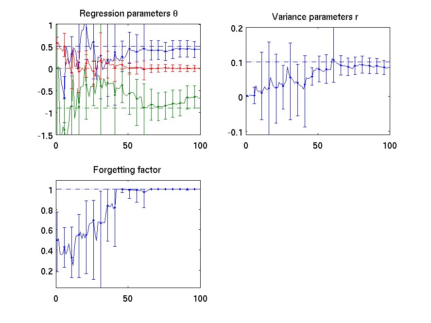
Note: error bars in this case are not directly comparable with those of previous examples. The MPF class implements the qbounds function as minimum and maximum of bounds in the considered set (even if its weight is extremely small). Hence, the bounds of the MPF are probably larger than it should be. Nevertheless, they provide great help when designing and tuning algorithms.
Matlab extensions of the Bayesian estimators
Similarly to the extension of pdf, the estimators (or filters) can be extended via prepared classmexBM in directory bdmtoolbox/mex/mex_classes.An example of such class is mexLaplaceBM in <toolbox_dir>/tutorial/userguide/laplace_example.m
Note that matlab-extended classes of mexEpdf, specifically, mexDirac and mexLaplace are used as outputs of methods posterior and epredictor, respectively.
In order to create a new extension of an estimator, copy file with class mexLaplaceBM.m and redefine the methods therein. If needed create new classes for pdfs by inheriting from mexEpdf, it the same way as in the mexLaplace.m example class.
For list of all estimators, see bdmtoolbox - List of available basic objects.
Generated on 2 Dec 2013 for mixpp by
 1.4.7
1.4.7