
BDM Use - System, Data, Simulation
This section serves as introduction to the scenario of data simulation. Since it is the simplest of all scenarios defined in BDM Use - Introduction it also serves as introduction to configuration of an experiment (see User Infos and their use) and basic decision making objects (bdm::RV and bdm::DS).
All experiments are demonstrated on mex file simulator, which is also available as a standalone application.
Table of contents:
ug_sim_config
ug_sim
ug_memds
ug_rvs
ug_rv_connect
ug_pdfds
ug_arx_sim
ug_ini
ug_store
ug_sim_config
Configuration file (or config structure) is organized as a tree of information. High levels represent complex structures, leafs of the tree are basic data elements such as strings, numbers or vectors.
Specific treatment was developed for objects. Since BDM is designed as object oriented library, the configuration was designed to honor the rule of inheritance. That is, offspring of a class can be used in place of its predecessor. Hence, objects (instances of classes) are configured by a structure with compulsory field class. This is a string variable corresponding to the name of the class to be used. This information is stored in Matlab structures (or objects, see section on Matlab extensions).
Advanced users can find more information in (User Infos and their use).
First experiment
The first experiment that can be performed is:DS.class='MemDS'; DS.Data =[1 2 3 4 5 6];
The code above is the minimum necessary information to run scenario simulator in Matlab. To actually do so, make sure that Matlab paths are correctly set, as described in BDM Use - Installation.
The expected result for Matlab is:
>> M=simulator(DS)
M =
ch0: [6x1 double]
All that the simulator did was actually copying DS.Data to M.ch0. Explanation of the experiment and the logic used there follows.
ug_sim
In standard system theory, the system is typically illustrated graphically as: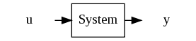
u typically denotes input and y denotes output of the system. A causal dependence between input and output is typically presumed.
We are predominantly concerned with discrete-time systems, hence, we will add indices  to both input and output,
  and
and  . We presume that the causal dependence is comes before .
One of the definition of a system is that system is a "set of variables observed on a part of the world". Under this definition system is understood as generator of data. This definition may be a considered too simplistic, but it serves well as a description of what software object DataSource is.
DataSource is an object that is essentially able to:
- return data observed at time
 ,
, - perform one a time step.
- describe what these data are, via class RV, introduced in ref Marginalization and conditioning,
- store log of its activity into dedicated logger.
No further specification, e.g. if the data are pre-recorded or computed on-the-fly, are given. For a list of available DataSources, see ...
ug_memds
The first experiment run in First experiment was actually an instance of DataSource of pre-recorded data that were stored in memory, i.e. the bdm::MemDS class.Operation of such object is trivial, the data are stored as a matrix and the general operations defined above are specialized as follows:
- data observed at time are columns of the matrix, getdata() returns current column,
- time step itself is performed by increasing the column index,
- each row is named as "ch0","ch1",...
This is the default behavior. It can be customized using the UI mechanism. Full list of options is:
DS.class = 'MemDS'; DS.Data = (...); // Data matrix or data vector --- optional --- DS.drv = RV({"ch0",...} ); // Identification how rows of the matrix Data will be known to others DS.time = 0; // Index of the first column to user_info,
Fields time denotes the first record to start counting from. Field drv is a the one that specifies identification of the data elements, (point 3. of the general requirements of a DataSource).
All optionals fields will be filled by default values, it this case:
DS.drv = RV({'ch0'},1,0);
DS.time = 0;
ug_rvs
RV stands forrandom variable which is a description of random variable or its realization. However, this object serves as general descriptor of fields in vectors of data.It is used for:
- description of RV in pdfs, ways how to define marginalization and conditioning,
- connection between source of data and computational objects that use them,
- connection time, more exactly time shift from , defaults to 0.
For example, the estimators will request the data from the above mentioned data source by asking for rv 'ch0'. If a more meaningful names are available, the fields drv can be added to read:
DS.class='MemDS';
DS.Data =[1 2 3 4 5 6];
DS.drv = RV('y');
ug_rv_connect
results of an experiment can be stored in many ways. This functionality was abstracted into a class called logger. Exact form of the stored results is chosen by choosing appropriate class. For example,stdlog writes all output in the console, dirfilelog writes all data in the dirfilelog format for high-speed data processing, mexlog writes data into Matlab structure. The mexlog is the default option in bdmtoolbox.
Connection between computational blocks and loggers is controlled by structure called log_level which governs the level of details to be logged. A standard Data source has two levels, logdt and logut which means "log all outputs, dt" and "log all inputs, ut". Readers familiar with Simulink environment may look at the RV as being unique identifiers of inputs and outputs of simulation blocks. The inputs are connected automatically with the outputs with matching RV. This view is however, very incomplete, RV have more roles than this.
ug_pdfds
For example, we would like to simulate a random Uniform distributed noise on interval <-1,1>. This is achieved by plugging an object representing uniform pdf into general simulator of independent random samples, pdfDS. Uniform density is implemented as class bdm::euni, which is created from the following structure:U.class='euni';
U.rv = RV({'a'});
U.high = 1.0;
U.low = -1.0;
![\[ f(a) = \mathcal{U}(-1,1) \]](form_139.png)
The datasource itself, i.e. the instance of EpdfDS can be then configured via:
DS.class = 'pdfDS';
DS.pdf  = U;
U is the structure defined above.
Contrary to the previous example, we need to tell to algorithm simulator how many samples from the data source we need. This is configured by variable experiment.ndat. The configuration has to be finalized by:
experiment.ndat = 10;
M=simulator(DS,experiment);
The result is as expected in field M.DS_dt_a the name of which corresponds to results form "datasouce" / "output_dt" / "name given in U.rv".
If the task was only to generate random realizations, this would indeed be a very clumsy way of doing it.
However, the power of the proposed approach will be revealed in more demanding examples, one of which follows next.
By default, data from this datasouce will be named after the rvs in given by the pdfs. When pdf with no rv is used, drv of the data source is set again to 'ch0'.
ug_arx_sim
Consider the following autoregressive model:
![\[ f(y_t|y_{t-3},u_{t-1}) = \mathcal{N}( a y_{t-3} + b u_{t-1}, r) \]](form_140.png)
where  are known constants, and
  is known variance.
We need to handle two issues:
- extra unsimulated variable
 ,
, - time delays of the values.
The first issue can be handled in two ways. First, can be considered as input and as such it could be externally given to the datasource. This solution is used in scenario closedloop. However, for the simulator scenario we will apply the second option, that is we complement  by extra pdf:
![\[ f(u_t) = \mathcal{N}(0, r_u) \]](form_147.png)
where  is another known constant. Thus, the joint density is now:
![\[ f(y_{t},u_{t}|y_{t-3},u_{t-1}) = f(y_{t}|y_{t-3},u_{t-1})f(u_{t}) \]](form_149.png)
and we have no need for input since the datasource have all necessary information inside. All that is required is to store them and copy their values to appropriate places.
That is done in automatic way (via bdm::datalink_buffered). The only issue a user may need to take care about is the missing initial conditions for simulation. By default these are set to zeros. Using the default values, the full configuration of this system is:
y = RV({'y'});
u = RV({'u'});
fy.class = 'mlnorm\<ldmat\>';
fy.rv    = y;
fy.rvc   = RV({'y','u'}, [1 1], [-3, -1]);
fy.A     = [0.5, -0.9];
fy.const = 0;
fy.R     = 0.1;
fu.class = 'enorm\<ldmat\>';
fu.rv    = u;
fu.mu    = 0;
fu.R     = 0.2;
DS.class = 'pdfDS';
DS.pdf.class  = 'mprod';
DS.pdf.pdfs  = {fy, fu};
Explanation of this example will require few remarks:
- class of the
fyobject is 'mlnorm<ldmat>' which is Normal pdf with mean value given by linear function, and covariance matrix stored in LD decomposition, see bdm::mlnorm for details. - naming convention 'mlnorm<ldmat>' relates to the concept of templates in C++. For those unfamiliar with this concept, it is basically a way how to share code for different flavors of the same object. Note that mlnorm exist in three versions: mlnorm<ldmat>, mlnorm<chmat>, mlnorm<fsqmat>. Those classes act identically the only difference is that the internal data are stored either in LD decomposition, choleski decomposition or full matrices, respectively.
- the same concept is used for enorm, where enorm<chmat> and enorm<fsqmat> are also possible. In this particular use, these objects are equivalent. In specific situation, e.g. Kalman filter implemented on Choleski decomposition (bdm::KalmanCh), only enorm<chmat> is approprate.
- class 'mprod' represents the chain rule of probability, see Conditioned densities.
The code above can be immediately run, using the same execution sequence of estimator as above.
ug_ini
When zeros are not appropriate initial conditions, the correct conditions can be set using additional commands:DS.init_rv = RV({'y','y','y'}, [1,1,1], [-1,-2,-3]);
DS.init_values = [0.1, 0.2, 0.3];
The values of init_values will be copied to places in history identified by corresponding values of init_rv. Initial data is not checked for completeness, i.e. values of random variables missing from init_rv (in this case all occurrences of ) are still initialized to 0.
ug_store
If the simulated data are to be analyzed off-line it may be advantageous to store them and use later on. This operation is straightforward if the class of logger used in thesimulator is compatible with some datasource class.
For example, the output of MemDS can be stored as an .it file (filename is specified in configuration structure) which can be later read by bdm::ITppFileDS.
In Matlab, the output of mexlog is a structure of vectors or matrices. The results can be saved in a Matlab file using:
Data=[M.y; M.u];
drv = RVjoin({y,u});
save pdfds_results Data drv
mxDS.class   = 'MemDS';
mxDS.Data    = 'Data';
mxDS.drv     = drv;
For list of all DataSources and loggers, see bdmtoolbox - List of available basic objects
Generated on 2 Dec 2013 for mixpp by
 1.4.7
1.4.7