BDM Use - System, Data, Simulation

This section serves as introdustion to the scenario of data simulation. Since it is the simpliest of all scenarios defined in user_guide0 it also serves as introduction to configuration of an experiment (see User Infos and their use) and basic decision making objects (bdm::RV and bdm::DS).

All experiments are demonstarted on scenario simulator which can be either standalone application or mex file (simulator.mex**).

Configuration of an experiment

Configuration file (or config structure) is organized as a tree of information. High levels represent complex structures, leafs of the tree are basic data elements such as strings, numbers or vectors.

Specific treatment was developed for objects. Since BDM is designed as object oriented library, the configuration was designed to honor the rule of inheritance. That is, offspring of a class can be used in place of its predecessor. Hence, objects (instances of classes) are configured by a structure with compulsory field class. This is a string variable corresponding to the name of the class to be used.

The configuration has two possible options:

configuration file using syntax of libconfig (see User Infos and their use),
matlab structure. For the purpose of tutorial, we will use the matlab notation. These two options can be mutually converted from one to another using prepared mex files: config2mxstruct.mex and mxstruct2config.mex. Naturally, these scripts require matlab to run. If it is not available, manual conversion is relatively trivial, the major difference is in using different types of brackets (User Infos and their use)

First experiment

The first experiment that can be performed is:

DS.class='MemDS';
DS.Data =[1 2 3 4 5 6];

which can be found in file bdmtoolbox/tutorials/userguide/memds_example.m.

The code above is the minimum necessary information to run scenario simulator in matlab. To actually do so, make sure that matlab can find the simulator.mex file, e.g. by running:

>> addpath _path_to_/bmtoolbox/mex/

The expected result for Matlab is:

>> M=simulator(DS)

M = 

    ch0: [6x1 double]

If you see this result, you have configured BDM correctly and you have sucessfully run you first experiment. In other cases, please check your installation, BDM Use - Installation. All that the simulator did was actually copying DS.Data to M.ch0. Explanation of the experiment and the logic used there follows.

Systems and DataSources

In standard system theory, the system is typically illustrated graphically as: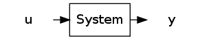

Where u typically denotes input and y denotes output of the system. A causal dependence between input and output is typically presumed.

We are predominantly concerned with discrete-time systems, hence, we will add indeces $ _t $ to both input and output, $ u_t $ and $ y_t $ . We presume that the causal dependence is $ u_t $ comes before $ y_t $ .

One of the definition of a system is that system is a "set of variables observed on a part of the world". Under this definition system is understood as generator of data. This definition may be a considered too simplistic, but it serves well as a description of what software object DataSource is.

DataSource is an object that is essentially:

able to return data observed at time , (bdm::DS::getdata()),
able to perform one a time step, (bdm::DS::step()).
able to describe what these data are, (bdm::DS::_drv()),

No fruther specification, e.g. if the data are pre-recorded or computed on-the-fly, are given. Specific behaviour of various DataSources is implemented as specialization of the root class bdm::DS.

DataSource of pre-recorded data -- MemDS

The first experiment run in first was actually an instance of DataSource of pre-recorded data that were stored in memory, i.e. the bdm::MemDS class.

Operation of such object is trivial, the data are stored as a matrix and the general operations defined above are specialized as follows:

data observed at time are columns of the matrix, getdata() ruturns current column,
time step itself is performed by increasing the column index,
each row is named as "ch0","ch1",...

This is the default bahavior. It can be customized using the UI mechanism. When the object of class MemDS is created it calls method bdm::MemDS::from_setting() and the input structure is parsed for settings. All available settings are documented in the method, see bdm::MemDS::from_setting(). The options are:

DS.class = 'MemDS';
DS.Data = (...);            // Data matrix or data vector
        --- optional ---
DS.drv = RV({"ch0",...} ); // Identification how rows of the matrix Data will be known to others
DS.time = 0;               // Index of the first column to user_info,
DS.rowid = [1,2,3...];     // ids of rows to be used

The compulsory fields are listed at the beginning; the optional fields are separated by string "--- optional ---".

Fields time and rowid are self-explanatory. Field drv is a the one that specifies identification of the data elements, (point 3. of the general requirements of a DataSource).

All optionals fields will be filled by default values, it this case:

DS.drv  = RV({'ch0'},1,0);
DS.time = 0;
DS.rowid = [1];

Where the first line specifies a universal identification structure: random variable (bdm::RV).

What is RV and how to use it

RV stands for random variable which is a description of random variable or its realization. This object playes role of identifier of elements of vectors of data (in datasources), expected inputs to functions (in pdfs), or required results (operations conditioning).

Mathematical interpretation of RV is straightforward. Consider pdf $ f(a)$ , then $ a $ is the part represented by RV. Explicit naming of random variables may seem unnecessary for many operations with pdf, e.g. for generation of a uniform sample from <0,1> it is not necessary to specify any random variable. For this reason, RV are often optional information to specify. However, the considered scenanrio simulator is build in a way that requires RV to be given.

In software, RV has three compulsory properties:

name, unique identifier, two RV with the same name are considered to be identical
size, size of the random variable, if not given it is assumed to be 1,
time, more exactly time shift from , defaults to 0. For example, scalar is encoded as (name='x',sizes=1,time=-2). Each RV stores array of these elements, hence RV with:
```
 names={'a', 'b'};
 sizes=[ 2 , 3];
 times=[-1, 1];
```
denotes 5-dimensional vector .

Algebra on RVs

Algebra on RVs (adding, searching in, subtraction, intersection, etc.) is implemented, see bdm::RV.

For convenience in Matlab, the following operations are defined:

RV(names,sizes,times) creates configuration structure for RV,
RVjoin(rvs) joins configuration structures for array of RVs rvs=[rv1,rv2,...],
RVtimes(rvs,times) assign times to corresponding rvs.

See examples in bdmtoolbox/tutorial/userguide

ug_rv_connect

The simulator scenario connects the DataSource to second basic class of BDM, bdm:logger. The logger is a class that take care of storing results -- in this case, results of simulation. The connection between these blocks is done automatically. The logger stores results of simulations under the names specified in drv. Readers familiar with Simulink environment may look at the RV as being unique identifiers of inputs and outputs of simulation blocks. The inputs are connected automatically with the outputs with matching RV. This view is however, very incomplete, RV have more roles than this.

Loggers for flexible handling of results

Loggers are universal objects for storing and manipulating the results of an experiment. Similar to DataSource, every logger has to provide basic functionality:

initialize its storage (bdm::logger.init()),
assign a connection point to each interested object (bdm::logger.logadd()),
accept data to be logged to given connection (bdm::logger.logit()),
finalize the storage when experiment is finished.

These abstarct operations can be specialized in many ways. For example, storing all results in memory and writing them to disc when finished (bdm::memlog), storing data in a matlab structure (bdm::mexlog), writing them out in ascii (bdm::stdlog) or more sophisticated buffered output to harddrive (bdm::dirfilelog).

Since all experiments are performed in matlab, the default mexlog class will be used. However, the way how the results are to be stored can be configured using configuration structure filled by fields from from_setting of the chosen logger, and passing it as third argument to simulator.

Class inheritance and DataSources

As mentioned above, the scenario simulator is written to accept any datasource (i.e. any offspring of bdm::DS). For full list of offsprings, click see Classes > Class Hierarchy.

At the time of writing this tutorial, available datasources are bdm::DS

bdm::EpdfDS
bdm::MemDS
- bdm::FileDS
  - bdm::CsvFileDS
  - bdm::ITppFileDS
bdm::MpdfDS
bdm::stateDS

The MemDS has already been introduced in the example in memds. However, any of the classes listed above can be used to replace it in the example. This will be demonstrated on the EpdfDS class.

Brief decription of the class states that EpdfDS "Simulate data from a static pdf (epdf)". The static pdf means unconditional pdf in the sense that the random variable is conditioned by numerical values only. In mathematical notation it could be both $ f(a) $ and $f(x_t |d_1 \ldots d_t)$ . The latter case is true only when all $ d $ denotes observed values.

For example, we wish to simulate realizations of a Uniform pdf on interval <-1,1>. This is achieved by plugging an object representing uniform pdf into general simulator of independent random samples, EpdfDS. Uniform density is implemented as class bdm::euni. An instance of euni can be again created method from_setting, in this case bdm::euni.from_setting(). Using documentation we define it with the following code:

U.class='euni';
U.rv   = RV({'a'});
U.high = 1.0;
U.low  = -1.0;

which encodes information:

$f(a) = \mathcal{U}(-1,1)$

The datasource itself, i.e. the instanc of EpdfDS can be then configured via:

DS.class = 'EpdfDS';
DS.epdf  = U;

where U is the structure defined above.

Contrary to the previous example, we need to tell to algorithm simulator how many samples from the data source we need. This is configured by variable experiment.ndat. The configuration has to be finalized by:

experiment.ndat = 10;
M=simulator(DS,experiment);

The result is as expected in field M.a the name of which corresponds to name of U.rv .

If the task was only to generate random realizations, this would indeed be a very clumsy way of doing it. However, the power of the proposed approach will be revelead in more demanding examples, one of which follows next.

Simulating autoregressive model

Consider the following autoregressive model:

$f(y_t|y_{t-3},u_{t-1}) = \mathcal{N}( a y_{t-3} + b u_{t-1}, r)$

where $ a,b $ are known constants, and $ r $ is known variance.

Direct application of EpdfDS is not possible, since the pdf above is conditioned on values of $y_{t-3}$ and $u_{t-1}$ . We need to handle two issues:

extra unsimulated variable ,
time delayes of the values.

The first issue can be handled in two ways. First, $ u $ can be considered as input and as such it could be externally given to the datasource. This solution is used in scenario closedloop. However, for the simulator scenario we will apply the second option, that is we complement 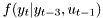$f(y_{t}|y_{t-3},u_{t-1})$ by extra pdf:

$f(u_t) = \mathcal{N}(0, r_u)$

where $ r_u $ is another known constant. Thus, the joint density is now:

$f(y_{t},u_{t}|y_{t-3},u_{t-1}) = f(y_{t}|y_{t-3},u_{t-1})f(u_{t})$

and we have no need for input since the datasource have all necessary information inside. All that is required is to store them and copy their values to appropriate places.

That is done in automatic way using dedicated class bdm::datalink_buffered. The only issue a user may need to take care about is the missing initial conditions for simulation. By default these are set to zeros. Using the default values, the full configuration of this system is:

y = RV({'y'});
u = RV({'u'});

fy.class = 'mlnorm<ldmat>';
fy.rv    = y;
fy.rvc   = RV({'y','u'}, [1 1], [-3, -1]);
fy.A     = [0.5, -0.9];
fy.const = 0;
fy.R     = 0.1;


fu.class = 'enorm<ldmat>';
fu.rv    = u;
fu.mu    = 0;
fu.R     = 0.2;

DS.class = 'MpdfDS';
DS.mpdf.class  = 'mprod';
DS.mpdf.mpdfs  = {fy, epdf2mpdf(fu)};

Explanation of this example will require few remarks:

class of the fy object is 'mlnorm<ldmat>' which is Normal pdf with mean value given by linear function, and covariance matrix stored in LD decomposition, see bdm::mlnorm for details.
naming convention 'mlnorm<ldmat>' relates to the concept of templates in C++. For those unfamiliar with this concept, it is basicaly a way how to share code for different flavours of the same object. Note that mlnorm exist in three versions: mlnorm<ldmat>, mlnorm<chmat>, mlnorm<fsqmat>. Those classes act identically the only difference is that the internal data are stored either in LD decomposition, choleski decomposition or full matrices, respectively.
the same concept is used for enorm, where enorm<chmat> and enorm<fsqmat> are also possible. In this particular use, these objects are equivalent. In specific situation, e.g. Kalman filter implemented on Choleski decomposition (bdm::KalmanCh), only enorm<chmat> is approprate.
class 'mprod' represents the chain rule of probability. Attribute mpdfs of its configuration structure is a list of conditional densities. Conditional density is represented by class mpdf and its offsprings. Class RV is used to describe both variables before conditioning (field rv ) and after conditioning sign (field rvc).
due to simplicity of implementation, mprod accept only conditional densities in the field mpdfs. Hence, the pdf must be converted to conditional density with empty conditioning, $f(u_t| \{\})$ . This is achieved by calling function epdf2mpdf which is only a trivial wrapper creating class bdm::mepdf.

The code above can be immediatelly run, usin the same execution sequence of estimator as above.

Initializing simulation

When zeros are not appropriate initial conditions, the correct conditions can be set using additional commands (see bdm::MpdfDS.from_setting() ):

DS.init_rv = RV({'y','y','y'}, [1,1,1], [-1,-2,-3]);
DS.init_values = [0.1, 0.2, 0.3];

The values of init_values will be copied to places in history identified by corresponding values of init_rv. Initial data is not checked for completeness, i.e. values of random variables missing from init_rv (in this case all occurences of $ u $ ) are still initialized to 0.

Storing results of simulation

If the simulated data are to be analyzed off-line it may be advantageous to store them and use for later use. This operation is straightforward if the class of logger used in the simulator is compatible with some datasource class.

For example, the output of MemDS can be stored as an .it file (filename is specified in configuration structure) which can be later read by bdm::ITppFileDS.

In matlab, the output of mexlog is a structure of vectors or matrices. The results can be saved in a matlab file using:

Data=[M.y; M.u];
drv = RVjoin({y,u});
save mpdfds_results Data drv

Such data can be later provided e.g. by MemDS

mxDS.class   = 'MemDS';
mxDS.Data    = 'Data';
mxDS.drv     = drv;